This online appendix provides complete mathematical derivations for all numbered equations in the main paper. The appendix is organized to mirror the structure of the paper, presenting step-by-step derivations, highlighting key mathematical techniques, and referencing computational implementations for verification.
Contents:
Section 3: Benchmark Model (Equations 1-15)
Section 4: Social Efficiency Analysis (Equations 16-21)
Section 5: Extended Model with Institutions (Equations 22-27)
Section 6: Applications and Extensions (Equations 28-43)
The paper’s symbol table, with a column added for the corresponding name in the
enclose
package — so a symbol here can be traced to the code that computes it.
Symbol
Meaning
Effect of an increase
Key thresholds
In code
θ
TFP gain on enclosed land (θ=Ae/Ac)
Raises the return to enclosing; crossing θHμ switches decisions from complements to substitutes, and the risk from over- to under-enclosure
θH=1/α; θ=1 separates progressive from regressive enclosure
th
A
Baseline TFP
Enters only as c/A: shifts every locus down by the same vertical distance
—
(absent — see below)
α
Labor share (Cobb–Douglas)
Lowers θH=1/α, shrinking the race-prone complements region
—
alp, default loci.ALP
lˉ=Lˉ/Tˉ
Population density
Smooth te↑ if θ>θH; a jump at lˉggd if θ<θH
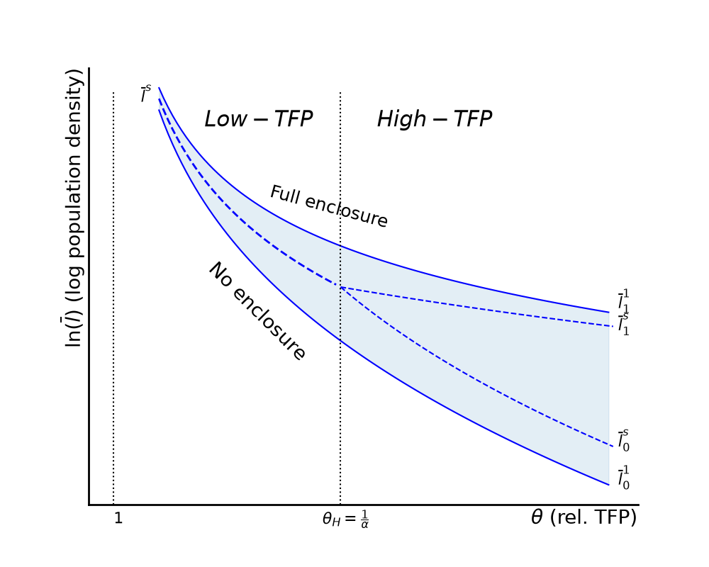
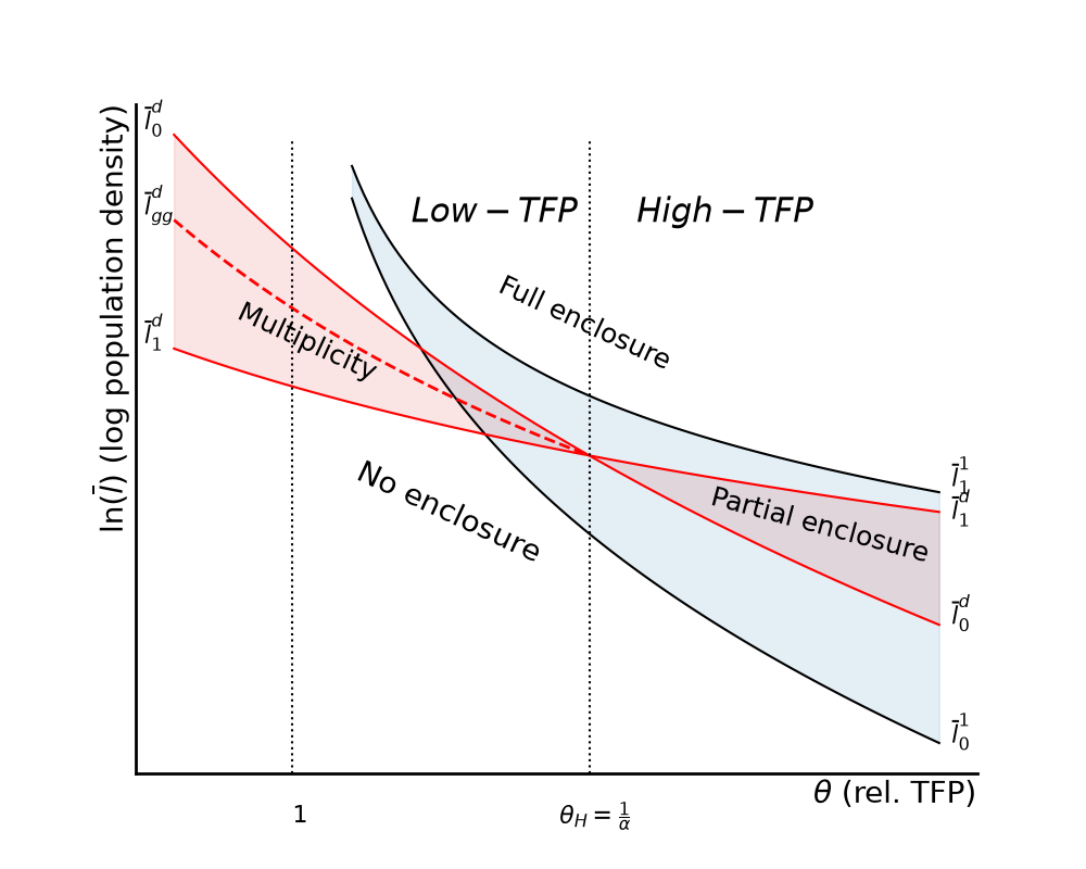
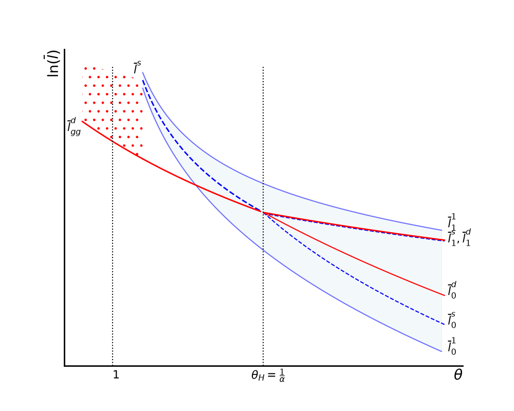
Loci lˉ01,lˉ11,lˉ0d,lˉ1d,lˉggd,lˉs,…
lbar; loci return lnlˉ
c
Enclosure cost per unit land
Shifts every locus up by the same vertical distance — geometrically identical to the economy’s point moving down
Enters all loci as c/A, each scaling as (c/A)1/α
c, default loci.C
te,le
Shares of land, labor in the enclosed sector
—
—
te, model.le
μ∈[0,1]
Community capacity to regulate commons access
Shrinks labor misallocation and moves θHμ left toward 1; under-enclosure shrinks, but over-enclosure expands if τ=0
μ=1: no misallocation; θHμ=α1−μα1−α
mu
τ∈[0,1]
Compensation/resistance power of customary users
Raises the density needed before enclosure pays; over-enclosure shrinks, under-enclosure expands
τ=1: “trade”; τ=0: “raid”
tau
Also used in this appendix, beyond the paper’s table:
Symbol
Meaning
In code
Λμ=(αθ/Aμ)1/(1−α)
Enclosed-to-commons labor intensity; Λo=θ1/(1−α) is the planner’s
model.Lambda(th, alp, mu), loci.lam_mu
Aμ=1−μ(1−α)
Share of the commons average product labor retains, eq. (37)
manufacturing.commons_wedge
θHμ
Where Λμ=1: enclosure switches labor-extensive to labor-intensive
model.theta_H(alp, mu)
θτ=τ1−α(Aμ/α)α
Below it enclosure earns less than the compensation owed, at any density — eq. (27b)
loci.theta_tau(alp, mu, tau)
Tˉ,Lˉ,Kˉ
Total land, labor, capital endowments; tˉ=Tˉ/Lˉ, kˉ=Kˉ/Lˉ
tbar, lbar, kb
lc,lm
Labor shares in the commons and in manufacturing (§6.4)
manufacturing.labor_share
β∈(0,1), p>0
Manufacturing labor share and relative price (§6.4)
We begin by establishing the production technology and key relationships. Production in both enclosed and unenclosed sectors follows Cobb-Douglas technology:
This decomposition is crucial: it shows that average product exceeds marginal product by the amount MPT⋅(T/L), which represents the possession rent that labor captures under open access when it must occupy land.
In the unenclosed (common) sector under open access, labor captures the average product (not marginal product) because workers must possess land to produce:
The key difference from (3) is the α multiplier on the left-hand side, reflecting that labor earns only its marginal product in the enclosed sector but captures the average product in the commons.
Equation (10): Labor Reaction Function (Decentralized)¶
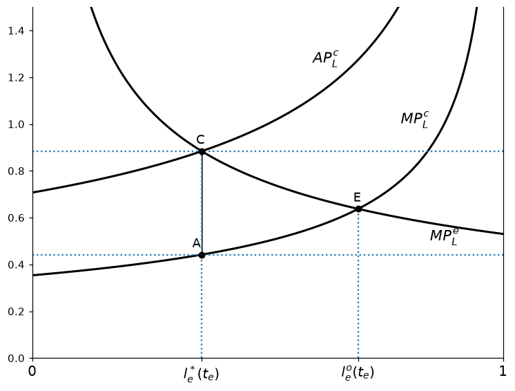
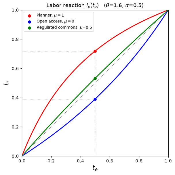
Critical Distinction: Under decentralized enclosure with open-access commons, Λ=(αθ)1−α1 whereas the planner uses Λo=θ1−α1. Since α<1, we have Λ<Λo, meaning the decentralized economy allocates less labor to enclosed land than is socially optimal (for any given te). This is the labor misallocation at the heart of the inefficiency.
Equation (11): Private Return to Enclosure (General Form)¶
which is the form used in the code. In the multiplicity region Λ<1 and αθ<1, so both the numerator and the denominator are positive.
Note: No special functions are needed — the integrand is a power of a linear function of te. (Earlier versions of this appendix stated that the evaluation involves a beta function and requires numerical integration. Both were incorrect; the closed form above is elementary, and is what the accompanying code has always used.)
[End of Section 3]
Section 4: Social Efficiency of Private Enclosure Decisions¶
We now ask whether decentralized enclosure decisions are at least “second-best” efficient—that is, optimal given the constraint that labor is misallocated due to open access. A second-best (or constrained) planner respects the labor allocation le0(te) that emerges from decentralized labor markets but can control the enclosure rate te.
Note: Unlike the first-best z1(te)=lˉα(1+(Λo−1)te)1−α which is always concave, z0(te) can be either concave or convex depending on θ relative to θH=1/α.
Private Return (θFTeAlˉα): The rental income captured by the encloser. This is what drives private enclosure decisions.
Displaced Rents (−FTcAlˉα): The marginal product of land in the commons that is lost when a unit of land is enclosed. Private enclosers do not internalize this loss, creating a negative externality that leads to over-enclosure.
Labor Reallocation Effect ((θFLe−FLc)Alˉα⋅dtedle0): When land is enclosed, labor reallocates from the commons (where it earns average product) to the enclosed sector (where it earns marginal product). This reduces the efficiency cost of labor misallocation. Private enclosers don’t capture this benefit, creating a positive externality that leads to under-enclosure.
Supporting Calculations:
For Cobb-Douglas, we can compute explicit expressions:
These expressions show precisely how the three effects vary with te and parameters (θ,α).
Key Result: The private enclosure decision (r(te)=c) ignores both the displaced rents term and the labor reallocation term. Depending on which effect dominates, private enclosure can be excessive or insufficient relative to the second-best.
Figure 4:MPL, APL and the labor misallocation wedge.
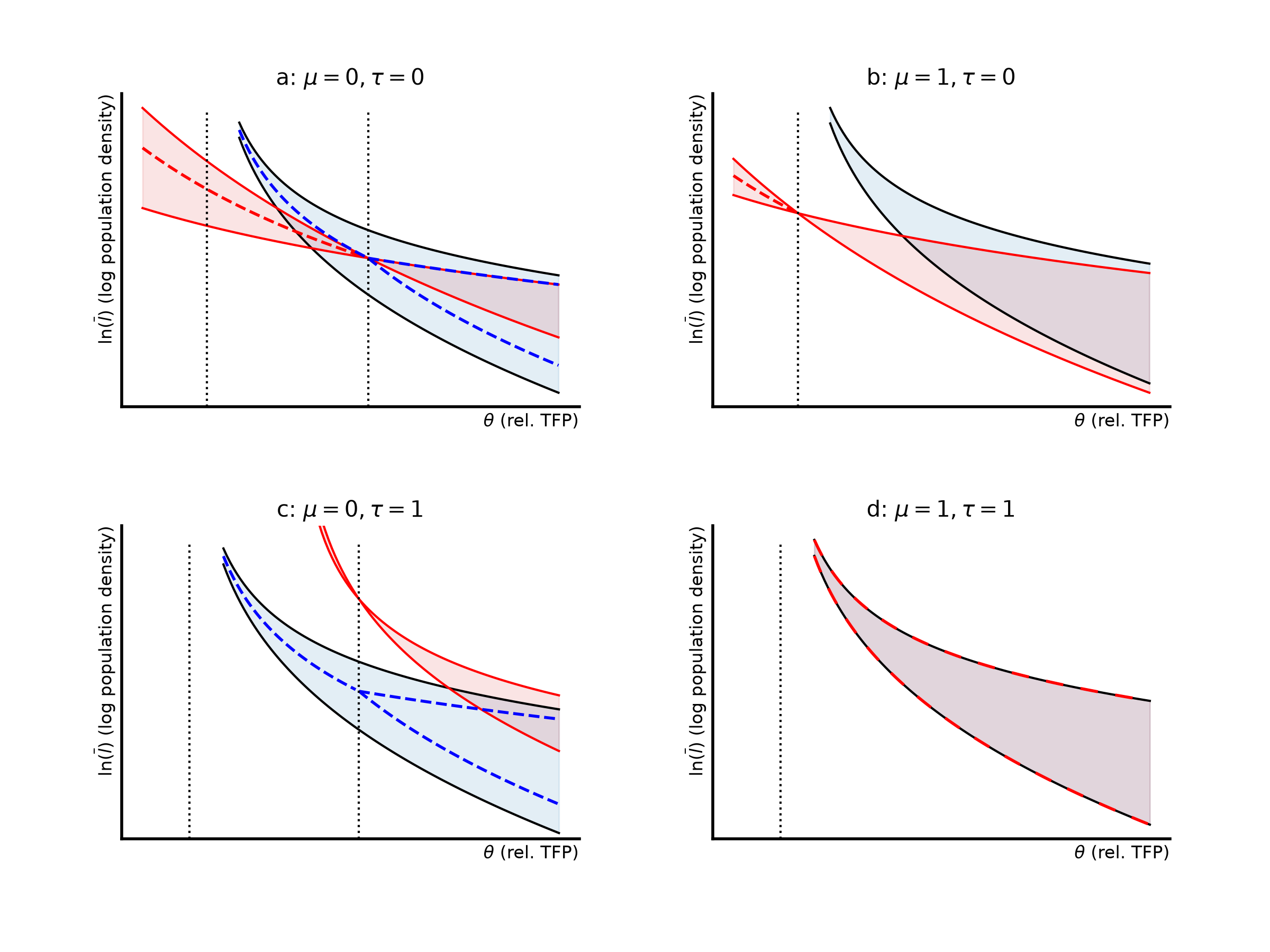
The baseline model assumes complete open access to unenclosed land (μ=0) and no compensation for displacement (τ=0). We now introduce institutional parameters to capture variations in governance quality and power relations.
Derivation:
Under imperfect governance of the commons, a worker who moves to the enclosed sector gives up not only their labor income but also a fraction (1−μ) of the possession rents they were capturing in the commons.
The wage in the enclosed sector is the marginal product of labor:
Scaling the displaced rents term by (1−τ) - compensation internalizes fraction τ
Scaling the labor reallocation term by (1−μ) - governance reduces misallocation
The labor reallocation effect now uses leμ(te) instead of le0(te), and the magnitude of the effect is proportional to (1−μ) since better governance reduces the initial misallocation.
Key Result: The wedge between private and social returns closes when:
μ=1ANDτ=1
With both parameters at 1, private incentives align with social optimum. However, improving only one dimension while holding the other fixed can worsen outcomes (second-best problem).
This generalizes equation (12) to allow for both governance quality (μ) and compensation requirements (τ).
Figure 6:Effects of varying μ and τ on equilibrium outcomes.
Equation (27a): Global Games Threshold under Governance and Compensation¶
Equations (13)–(14) generalize to the extended model by substituting (27) for (12), and so
does the selection criterion of equation (15). The multiplicity region does not disappear
when μ or τ is positive — it is θ<θHμ, which is non-empty for
every μ∈[0,1] — so a risk-dominance threshold continues to exist there and can be
written down.
The two rents in (27) share the same dependence on te, so they combine before integrating:
It is defined where θ<θHμandθΛμα>τ —
an interval, squeezed from the right by governance and from the left by compensation. The
second edge is derived below and is substantive rather than technical.
The governance wedge Aμ=1−μ(1−α) of equations (22)–(23) does not appear
as a separate factor here. Using Λμ1−α=αθ/Aμ, it enters
numerator and denominator alike and cancels, leaving μ to act only through
Λμ. This is specific to this locus: in the labor-market conditions of §5.1,
Aμ sets the level of what labor takes home and does not cancel.
Comparative statics. The two institutional parameters move the threshold in opposite
directions. Compensation raises it: τ enters only through (θΛμα−τ), so a larger τ shrinks the expected return and a higher density is needed to
trigger the cascade. Governance lowers it. Raising μ reduces Aμ, which raises
Λμ and hence the encloser’s return θΛμα — a regulated
commons pays labor its marginal rather than its average product, so the outside wage an
encloser must match is lower. At α=2/3, θ=0.9, τ=0:
μ
Aμ
Λμ
θΛμα
lnlˉggd
0.0
1.000
0.216
0.324
2.700
0.3
0.900
0.296
0.400
2.495
0.6
0.800
0.422
0.506
2.279
1.0
0.667
0.729
0.729
1.970
Better commons governance therefore makes the enclosure race easier to trigger, at the same
time as it shrinks the region in which a race is possible at all, since θHμ falls
from 1/α to 1 over the same range. The two effects work against each other, and
which dominates is a quantitative question.
Verification: (27a) was checked against symbolic integration, against numerical quadrature
of the payoff, and by reduction to the two one-sided forms already implemented in the code —
equation (15) extended in τ at μ=0, and the μ-extended form at τ=0.
Equation (27b): Where the Selection Threshold Ceases to Exist¶
The condition θΛμα>τ in (27a) has a closed-form boundary.
Setting the two equal and using Λμ1−α=αθ/Aμ:
Population density scales both the encloser’s gross return and the compensation owed, so
it cannot change the sign of their difference. Below θτ the expected net return
is negative at every density: the threshold does not move upward out of reach, it ceases
to exist.
This distinguishes the two obstacles to enclosure in the model:
how it enters
can density overcome it?
Enclosure cost c
a level charge per unit land
Yes. Rents scale with lˉα while c does not, so some density always suffices. This is why every locus is downward-sloping and finite.
Compensation τ
a proportional claim on displaced rents
No. It scales with the thing it taxes, so the comparison is density-free. Below θτ no density suffices.
The distinction matters for the Boserupian reading of the model. Rising population density
is the mechanism that drives an economy through every other threshold in the paper —
lˉ01, lˉ0d, lˉggd. Compensation is the one institution it cannot
push through. Cost-based protections for customary users — titling fees, registration
requirements, administrative friction — are eroded by population growth, because they are
levels. A compensation requirement is not, because it is a share.
Closure at the corner. Since θHμ=Aμ/α and
θτ=τ1−α(Aμ/α)α, the interval
(θτ,θHμ) is non-empty whenever τ<1 or μ<1, and empty
exactly at μ=τ=1, where both equal 1. So the coordination problem vanishes at
precisely the corner where the wedge closes: complete governance and complete compensation
not only align the decentralized loci with the planner’s (§5.3), they eliminate the
multiplicity that made equilibrium selection necessary in the first place. Neither parameter
achieves this alone — at μ<1 a multiplicity region survives even at τ=1, since
(Aμ/α)α<Aμ/α whenever Aμ/α>1.
Derivation:
Unlike competitive enclosers who take r(te) as given, a monopolist internalizes the effect of their enclosure decisions on the rental rate. Total profit is rental income minus enclosure costs.
Derivation: From π′(te)=r(te)+r′(te)te−c, evaluate at boundaries. The monopolist restricts enclosure below competitive levels when r′(te)<0 (high-TFP), as they internalize the rent-reducing effect of enclosure.
Figure 7:Monopolist’s enclosure decisions vs. competitive outcomes.
Derivation: The intra-agricultural condition is unchanged — equation (22) equalizes returns between enclosed land and the commons whatever else the economy contains — so the only modification is that the agricultural labor force is (1−lm) rather than 1. Following the steps of (23) with (1−lm) in place of 1 gives (36). The same expression with Λo in place of Λμ is the planner’s allocation, since μ=1 gives Λ1=Λo.
Everything below is stated in intensive form with tˉ=Tˉ/Lˉ and kˉ=Kˉ/Lˉ; factor-price levels carry the same density scaling as Section 3.
Derivation: From the Euler decomposition (8), APLc=MPLc+MPTc⋅(Tc/Lc), with MPLc=αAPLc and hence MPTc(Tc/Lc)=(1−α)APLc. Equation (22) says a worker leaving the commons forfeits the fraction μ of those possession rents, retaining (1−μ). Total commons income per worker is therefore
μ=0 recovers open access, where labor captures the whole average product; μ=1 gives the marginal product, which is the planner’s valuation.
Aμ is stated separately from Λμ because the two are not substitutes: Λμ governs the slope of the labor allocation, Aμ the level of what labor earns, and they enter subsequent expressions independently. The distinction is invisible in the two-sector model, where the level cannot affect an allocation that is agricultural regardless.
and wc=Aμ⋅APLc by (37). Equivalently, working from the enclosed side, θMPLe=αθtˉ1−α(te/leμ)1−α=αθΛμ−(1−α)tˉ1−α(1+(Λμ−1)te)1−α(1−lm)−(1−α), and αθΛμ−(1−α)=Aμ by the definition of Λμ in (23). The two routes agree, as they must.
Note that at μ=0 the prefactor equals exactly 1, so the agricultural side can be written compactly as tˉ1−α(te/le0)1−α. That shorthand does not survive to μ>0, where the prefactor is Aμ and not 1.
Two properties pin the level and serve as checks:
At te=0, Λμ drops out and Ca=Aμtˉ1−α, so the planner’s and open-access curves differ by exactly α — one pays labor its average product, the other its marginal product.
At te=1 there is no commons, so μ cannot matter: Ca=AμΛμ1−αtˉ1−α=αθtˉ1−α for everyμ. Equivalently, full enclosure implements the planner’s inter-sectoral labor allocation for any θ — conditional on te, a qualification equation (40) makes essential.
Existence and uniqueness. The left side is continuous and strictly increasing on (0,1), from 0 to ∞. Hence (39) has exactly one solution for any Cm/Ca>0: the equilibrium exists and is unique for all admissible parameters, and a bracketed root-finder on (0,1) is guaranteed to converge.
Closed form when β=α. The exponents coincide and (39) becomes (1−lmlm)1−α=CaCm, so
For β=α equation (39) is transcendental and has no elementary solution.
Comparative static in te.∂Ca/∂te has the sign of (Λμ−1). Because the left side of (39) is increasing in lm, the manufacturing share rises exactly when Ca falls, so
— the opposite sign, an inversion easily lost. By (24), Λμ=1 exactly at θHμ, so enclosure accelerates structural transformation below that threshold, retards it above, and moves no labor at all at it. The knife-edge is exact. Equation (41) tabulates the consequences; note that θHμ is the same threshold that separates strategic complements from substitutes in (24), a coincidence taken up there.
Equations (36)–(39) condition on te. Restoring the planner’s choice of te, and applying the envelope theorem — at the planner’s allocation marginal products are already equal, so reallocating labor has no first-order effect and only the land-rent differential survives:
Derivation:dY/dte=θFTe−FTc=(1−α)tˉ1−α[θ(le/te)α−(lc/(1−te))α]. Substituting (36) at μ=1 gives le/te=Λo(1−lm)/Do and lc/(1−te)=(1−lm)/Do with Do=1+(Λo−1)te, and θΛoα=Λo1−αΛoα=Λo.
This is exactly z′(te) from Section 3 with the agricultural labor share (1−lm) in place of the whole labor force. Manufacturing changes the level but not the sign.
Two thresholds, not one. The sign of (40) is that of (Λo−1), i.e. of (θ−1) — note Λo, not Λμ. This margin turns at θ=1; the labor-allocation reversal of (39) turns at θHμ. They answer different questions — is enclosure worth doing versus which way does it push labor — and must not be conflated. Below θ=1 enclosure lowers output even at c=0; at θ=1 (40) is identically zero; above it the planner encloses while (40) exceeds ctˉ.
So teo=0 for every c>0 whenever θ≤1, however misallocated the decentralized economy’s labor is at te=0. That full enclosure reproduces the planner’s labor allocation does not make full enclosure optimal. At θ=1 in particular, the whole gain from enclosure is the repair of the commons distortion, which regulating the commons (μ→1) achieves at te=0 without incurring cTˉ.
The two thresholds therefore bracket a band, and the parameter space divides into three regimes:
Regime
Range
Enclosure socially desirable?
Effect on structural transformation
Enclosure game
A
θ<1
No (at any c>0)
Releases labor to manufacturing
Complements
B
1<θ<θHμ
Yes, if c small enough
Releases labor to manufacturing
Complements
C
θ>θHμ
Yes, if c small enough
Draws labor back into agriculture
Substitutes
Regime B is the configuration the conventional account of enclosure and industrialization presumes — enclosure both efficiency-improving and labor-releasing. By (41) its width is proportional to (1−μ), so it exists only to the extent that the commons is poorly governed, and closes entirely at μ=1. It is also wider the larger is land’s share (1−α). The conventional account is thus not a general property of enclosure but a feature of the open-access case, and one that yields an inverted comparative static: within B, the labor-release effect weakens as θ rises toward θHμ, so enclosures delivering the largest productivity gains should release the least labor.
The last column is not an additional assumption. By (12), rμ(te) is increasing in te exactly when Λμ<1 — the condition for strategic complementarity, and hence for the multiplicity that (15) resolves. By (39) that is also exactly the condition for enclosure to release labor. The two are the same inequality because both turn on whether enclosed land is more or less labor-hungry than the commons. Hence:
Wherever enclosure accelerates structural transformation, the enclosure game admits multiple equilibria; wherever it retards structural transformation, the equilibrium is unique.
Regimes A and B lie entirely inside the strategic-complements region and C entirely outside it. The enclosures relevant to industrialization are therefore precisely those whose extent is not pinned down by fundamentals alone.
Equation (42): Private Enclosure with Manufacturing and Compensation¶
Equations (40)–(41) describe what the planner would do. Restoring the decentralized enclosure condition (27) in the presence of manufacturing:
Derivation: With manufacturing present, the enclosed and commons labor–land ratios are Le/Te=Λμ(1−lm)lˉ/Dμ and Lc/Tc=(1−lm)lˉ/Dμ, with Dμ=1+(Λμ−1)te, by (36). Substituting into rμe=θ(1−α)A(Le/Te)α and rμc=(1−α)A(Lc/Tc)α and collecting terms gives (42). The marginal encloser takes lm and the wage as given, so lm enters as a level, not through a strategic term.
The factorization is worth pausing on. Manufacturing enters only through (1−lm)α — a scale factor common to both rentals, reflecting that a smaller agricultural labor force lowers the land–labor ratio and hence both rents equally. τ enters only the bracket. The planner’s counterpart, from (40), is the bracket [Λo−1]; since θΛμα=Λμ when μ=1, private and social margins coincide exactly at μ=1andτ=1, which is the condition stated in §5.3.
τ∗ is strictly increasing in both θ and μ. The second is a second-best tension in its own right: better commons governance raises Λμ and hence the enclosed-land rent, so improving governance makes enclosure harder to deter by compensation, even as it makes deterrence more worthwhile.
Setting τ∗=1 and solving gives the range over which full compensation binds at all:
Since θHμ≥1 and α<1, this lies strictly between 1 and θHμ and collapses to 1 at μ=1. Above it no admissible τ prevents enclosure, and compensation is a pure transfer with no allocative consequence. This splits regime B of (41) at (θHμ)α into a sub-range where a compensation requirement blocks enclosure and one where it does not.
τ moves neither threshold of (41). Appearing in neither production nor the planner’s objective, it cannot shift θHμ or the θ=1 margin. Its role is to select which te is reached, not what enclosure does once there: μ changes what enclosure would do, τ changes whether it happens.
Consequently the two instruments are complements rather than substitutes, and ∂Y/∂τ changes sign with μ. Requiring compensation without regulating the commons removes the repair of the labor misallocation that enclosure was accomplishing; requiring it with a regulated commons prevents enclosure that would merely expend c. This is the claim of §5.3, now with a second margin on which it operates. Worked numerical illustrations are in enclose/manufacturing.py.
Caveat. Any equilibrium te computed from the marginal condition alone is incomplete for θ<θHμ, where (15)'s refinement is needed to select among multiple equilibria.
[End of Section 6]
Interpretation of these results — the mapping from regimes to historical accounts of enclosure, the relation to dual-economy models, and the research agenda they suggest — is deliberately not developed here. See notes/manuf_paper_ideas.md in the project repository.
Commons average product APLc(te). The wage is Aμ⋅weq, per (37) — the two coincide only at μ=0
θ, α, lˉ, μ
zprime(te, th, alp, lbar, mu)
(6), (7), (19), (20)
Marginal benefit z′(te) or z0′(te)
θ, α, lˉ, μ
teopt(th, alp, c, lbar)
Lemma 1
Optimal enclosure rate (first-best)
θ, α, c, lˉ
tepvt(th, alp, c, lbar, mu)
Props 2-3
Private enclosure rate
θ, α, c, lˉ, μ
tepvt_g(th, alp, c, lbar, mu)
(15)
Global games refined equilibrium
θ, α, c, lˉ, μ
mple(te, le, a, th, lbar)
Supporting
Marginal product of labor (enclosed)
mpt(te, le, a, th, lbar)
Supporting
Marginal product of land
totalq(te, th, alp, lbar, mu)
Supporting
Total economy output
The three-sector extension of §6.4 lives in a separate module, enclose/manufacturing.py
in the open-enclose.github.io repository, with tests in tests/test_manufacturing.py:
Python Function
Equations
Purpose
Key Parameters
commons_wedge(alp, mu)
(37)
Governance wedge Aμ
α, μ
mpl_m(lm, p, kb, b)
(38)
MPLm, manufacturing side
p, kˉ, β
mpl_a(lm, te, tbar, alp, th, mu)
(38)
Agricultural return Aμ⋅APLc — a marginal product only at μ=1
α, θ, μ, te
labor_share(te, ...)
(39)
Equilibrium lm, bracketed solve
all
labor_share_closed_form(te, ...)
(39)
Exact lm at β=α; used as a test oracle
all
agricultural_labor(te, ...)
(36)
leμ(te) with manufacturing present
θ, α, μ
total_output(te, ...)
Supporting
Y/Lˉ at the equilibrium allocation, gross of c
all
planner_marginal_benefit(te, ...)
(40)
dY/dte at the planner’s allocation
α, θ, β, p
private_marginal_return(te, tau, ...)
(42)
rμe−τrμc with manufacturing
α, θ, β, μ, τ
compensation_threshold(th, alp, mu)
(43)
τ∗(θ,μ)
α, θ, μ
Equation (37) is the correction most worth checking against: it was absent from earlier
drafts of this material, which stated the μ=0 shorthand of (38) as though it held for
all μ. tests/test_manufacturing.py pins it by verifying the planner’s first-order
conditions against the primitive derivatives of the objective, independently of any
expression in §6.4.
Cobb-Douglas Properties: All derivations exploit homogeneity and the relationship between marginal and average products
Closed-Form Integration: The expectation in equation (15) — and its extension (27a) — integrates in closed form by the power rule; no quadrature or special functions are required
Root Finding: Interior solutions (equations 6, 7, 13, 14, 19, 20) are found by setting derivatives equal to costs
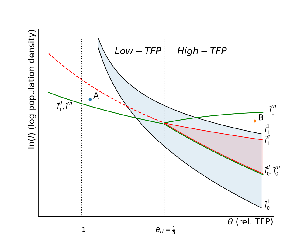
Parameter Space Partitioning: Threshold loci divide (θ,lnlˉ) space into regions