The benchmark model has one mobile factor moving between enclosed and unenclosed agriculture. Historically the interesting question is what enclosure did to the other margin: whether it released labor to industry. This page adds a manufacturing sector and asks exactly that — and finds the answer is not the one the standard narrative assumes.
1. Three sectors¶
Labor moves freely between manufacturing and agriculture, and within agriculture between enclosed and unenclosed land. Capital is specific to manufacturing, land to agriculture — an augmented specific-factors model, with the twist that land may be enclosed or not, which changes agricultural labor demand and hence labor supply to industry.
| Technology | Sector |
|---|---|
| Manufacturing | |
| Unenclosed agriculture | |
| Enclosed agriculture |
with labor adding up as .
2. Labor allocation within agriculture¶
Given a manufacturing share , the within-agriculture allocation is exactly the benchmark reaction function with the agricultural labor force shrunk to — equation (36):
Nothing about the enclosure margin changes; the whole three-sector extension enters through that one scaling factor. This is why the benchmark’s closed forms survive.
3. Where the manufacturing share settles¶
Labor moves until it earns the same everywhere, . Under open access the last of these is the commons average product, ; under perfect regulation it is the marginal product, . In general labor takes home the fraction
of the average product — its marginal product , plus the share of possession rents it still captures, . So and . Writing the two sides of the manufacturing/agriculture margin:
falls in and the agricultural return rises in it, so the two cross exactly once: the
equilibrium exists and is unique for any admissible parameters. (enclose.manufacturing
exploits this — it solves with a bracketed root-finder, which is guaranteed to converge,
rather than an initial-guess method that could wander.)
Rearranged, the condition is
which for is transcendental — there is no closed form, and the equilibrium must be found numerically. The one exception is , where the exponents coincide and it collapses to
That special case is worth keeping in view: it is the only fully solvable version, and it serves as an exact check on the numerical solver used everywhere else.
The constant-wage limit ()¶
The specification above gives manufacturing a fixed capital stock, so falls in and the wage stays endogenous. The opposite benchmark — manufacturing as a constant-returns sector absorbing unlimited labor at a fixed wage — is the corner of this same model. It is worth working out, because it isolates exactly which results depend on the wage being free to move.
At the manufacturing side of the margin loses its : . The equilibrium condition stops being a crossing condition and becomes a level condition on agriculture alone:
Agricultural employment no longer clears against manufacturing; it is pinned by and moves one-for-one with as land is enclosed, with manufacturing absorbing the residual. (Interior only while ; a low enough drives to zero and returns the economy to the two-sector benchmark.)
What it does to labor intensities. From the reaction function of §2, unenclosed labor per unit of unenclosed land is
and the condition above gives . The two factors cancel exactly: is constant in , and so is . Both land rents are constant, and so is the return to enclosing.
The consequence: . Enclosure decisions are then neither strategic complements nor substitutes — the dichotomy is degenerate, and with it go multiple equilibria, tipping, the property race, and the global-games refinement that selects among them. Enclosure collapses to a single comparison of a constant against : still all-or-nothing, but with no strategic interaction between enclosers and no coordination failure to resolve.
That makes the limit a clean diagnostic of what the wage feedback is doing in the benchmark. Every coordination result rests on one channel — enclosure displaces labor onto the commons, which depresses the commons return, which raises the return to enclosing. Give displaced labor somewhere else to go at an unchanged wage and the channel is cut at its first link.
What survives.
is untouched. It depends only on and , so the threshold separating labor-extensive from labor-intensive enclosure — and hence §6’s direction result, whether enclosure releases labor to industry or draws it back — holds exactly as stated.
The efficiency wedge remains. At commons labor still earns above its marginal product, so entry is still excessive, and an encloser who pays no compensation still fails to internalise displaced rents. Over-enclosure survives; what disappears is the cascade, not the externality.
And it is a knife-edge. is the only value at which the cancellation is exact. For any the manufacturing wage responds to , the two factors no longer cancel, and recovers its benchmark sign, that of — attenuated, monotonically in how elastic the outside option is, but qualitatively the benchmark’s. The results are therefore robust in the sense that matters: they require only that the outside option not be perfectly elastic.
4. Enclosure without any productivity gain¶
Set , so enclosure yields no technological improvement whatever, and compare an unenclosed economy with a fully enclosed one.
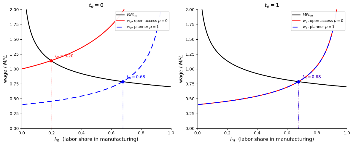
Figure 1:Labor market equilibrium before and after enclosure, at , , . Left: no land enclosed — the two agricultural curves stand in the ratio , since open access pays labor the commons average product and a planner its marginal product. Right: all land enclosed — the curves coincide, because there is no commons left for governance to apply to. The decentralized share moves from to ; the planner’s sits at 0.68 throughout.
Two facts about the right-hand panel generalise beyond this example. At there is no commons, so every worker is paid a marginal product whatever was, and regardless. Hence:
Full enclosure implements the planner’s inter-sectoral allocation, for any — conditional on . It does not follow that full enclosure is first best; see §5.
What varies with is where that allocation is, not whether enclosure reaches it.
So the decentralized economy does shift nearly half its workforce into manufacturing, and the shift owes nothing to productivity: by construction. But it is not a shift away from the optimum. The unenclosed economy was the misallocated one, holding labor on the land because the commons paid average rather than marginal product; enclosure removes that wedge and closes the gap exactly. Decentralized output rises 13.0% between the two panels, purely from reallocation.
Planner output, meanwhile, is identical in the two panels — 1.397 either way. That is the tell, and §5 makes it the argument: at enclosure buys a planner nothing at all. Everything it achieves here is the repair of a distortion, and repairs have alternatives.
The equilibrium wage nonetheless falls, from 1.14 to 0.79 — the Weitzman–Samuelson effect. It is worth being precise about what those two numbers are. At labor captures the whole average product of the commons; at it is paid a marginal product. The fall is a change in which of the two labor receives, not a fall in anyone’s productivity. Output and labor’s share move in opposite directions here, and the distributional loss is real — but it is not evidence that the inter-sectoral allocation got worse.
None of this is a welfare verdict on enclosure. What the example establishes is narrower: at this margin, in this case, the harm is not misallocation between agriculture and industry. §5 takes up the verdict itself.
5. Is enclosure worth its cost?¶
§4 held fixed and asked how labor is allocated. The planner also chooses , and that is a different margin with a different threshold. Adding it back:
By the envelope theorem the labor-reallocation terms vanish — the planner has already equalised marginal products, so shifting labor has no first-order effect — and all that survives is the land-rent differential :
This is the benchmark model’s with the agricultural labor share in place of the whole labor force. Manufacturing changes the level and not the structure — and in particular not the sign, which is the sign of , that is, of .
So:
| planner’s | ||
|---|---|---|
| negative — enclosure lowers output even at | 0 | |
| exactly zero at every | 0 for any | |
| positive | encloses while |
Full enclosure is first best only when and is small enough. For the planner does not enclose at all, no matter how badly the decentralized economy is misallocating labor at . The §4 result — that full enclosure reaches the planner’s labor allocation — is a statement about one margin, and does not carry to the other.
Enclosure as a second-best instrument¶
The case makes the distinction sharp. Three allocations, at , :
| output | |
|---|---|
| decentralized, no enclosure (, ) | 1.236 |
| decentralized, full enclosure (, ) | 1.397 |
| regulated commons, no enclosure (, ) | 1.397 |
Enclosure closes the entire 0.161 gap — and so does regulating the commons, at , for no enclosure cost at all. Enclosure is a second-best instrument here: it fixes the labor misallocation by abolishing the institution that caused it, which works, but pays for what governance would deliver directly. It beats doing nothing only while , and it never beats fixing the commons.
That is the reading the model actually supports, and it is not the enclosure-friendly one. Where enclosure raises output without raising productivity, it is substituting for an institutional reform, not accomplishing something reform could not.
Below ¶
For enclosure destroys land productivity as well as costing , so the planner’s answer is immediate. The decentralized economy is more interesting: the commons distortion is large enough that full enclosure still raises output for a range of below one — down to at these parameters — before the productivity loss overwhelms it. So there is a band, roughly , where enclosure raises decentralized output, lowers planner output, and is worth doing only if both is small and commons governance is unavailable.
Unlike , that lower crossover is not a clean knife-edge: it moves with , and (0.73 at ; 0.89 at ; 0.42 at ). It is a numerical feature of the example, not a result.
6. The effect reverses at ¶
The example above is not general — and the direction in which it generalises is the substantive finding on this page.
carries the factor , so the sign of is simply the sign of — note the inversion: the equilibrium condition’s left side rises in , so rises exactly when falls. (This is the reverse of §5’s enclosure margin, which does carry the sign of directly. Two margins, two signs.) The wedge does not interfere: it contains neither nor , so it moves the level of agricultural labor demand without touching its slope, and the result below holds for every . And holds exactly at
the same threshold that separates strategic complements from substitutes in the benchmark model. So:
— enclosure is labor-extensive, agricultural labor demand falls as rises, and labor is released into manufacturing. Enclosure accelerates structural transformation.
— enclosure is labor-intensive and pulls labor back into agriculture. Enclosure retards structural transformation.
— enclosure moves no labor at all.
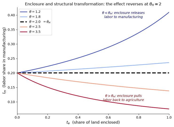
Figure 2:Manufacturing’s labor share as land is enclosed, for either side of . Below the threshold the curves rise, above it they fall, and at exactly the line is flat — the knife-edge is exact, not approximate.
The reading matters for economic history. The familiar account — enclosure freed labor for industry — is a claim about the low-TFP branch. Precisely where enclosure is most defensible on efficiency grounds, because it delivers a large productivity gain, it is least likely to release labor. The §4 example makes the point sharply: the case with the biggest labor release is the case with no productivity gain at all.
Governance moves the threshold¶
Since falls in — from at down to 1 at — better commons governance widens the region in which enclosure retards structural transformation. Where the commons is already well regulated, enclosure is more likely to draw labor back into agriculture than to release it.
This follows directly from the above, but its implications have not been worked through. It is stated here as a lead, not a result.
7. Socially optimal enclosure with manufacturing¶
The planner chooses to maximise
The two labor first-order conditions equate marginal value products across all three sectors, . The first gives back the benchmark planner’s reaction function scaled by , with ; the second, after substituting it, gives the agricultural side of the manufacturing margin as the general expression of §3 evaluated at , where . Both derivations are in online appendix §6.4, equations (36) and (38).
That leading is not decoration. Without it the planner’s labor demand is overstated by , the two curves in the §4 figure coincide in the left panel instead of the right, and the comparison in §4 comes out backwards.
The third first-order condition, in , is the enclosure margin — that is §5, where the envelope theorem reduces it to the land-rent differential alone.
The contrast with the decentralized economy is the same one as in the benchmark model: the private economy equates the enclosed sector’s marginal product to the unenclosed sector’s average product. The extra sector does not introduce a new distortion — it gives the existing one another margin to act on, and, as §4 shows, one that full enclosure happens to close. Whether closing it that way is worth doing is the separate question §5 answers, and usually the answer is no.
8. Status and open questions¶
The manufacturing price is exogenous. Endogenising it is the obvious next step and could overturn the partial-equilibrium comparative statics in §6.
§5 compares output, not welfare. It takes no view on the distributional shift from average- to marginal-product pay, which §4 shows moves opposite to output. Any actual welfare statement needs a weight on that, and this page does not supply one.
§5 derives the planner’s . The decentralized is still taken as given — closing that loop, with enclosers responding to a manufacturing outside option, is what would make this a paper rather than an extension. Expect the enclosure loci to move, since the outside option changes what the commons is worth.
§5’s second-best reading invites the obvious follow-up: if governance () and enclosure () are both costly instruments for the same distortion, what does the trade-off between them look like? The appendix’s belongs in that comparison too.
Whether enclosure raises measured aggregate TFP is worth computing explicitly. §4 suggests much of any such gain is composition: labor moving from a low-average-product commons into manufacturing, with no technology change anywhere.
The code behind every figure here is in enclose/manufacturing.py, with the uniqueness
property, the closed form, the reversal, the wedge and
§5’s enclosure margin (planner_marginal_benefit, total_output) all pinned by tests in
tests/test_manufacturing.py — the wedge by checking the planner’s first-order conditions
against the primitive derivatives of the objective above, the enclosure margin against a
numerical derivative of the value function.