This page walks through how the paper’s results are derived — the steps, the substitutions that make the algebra collapse, and the intuition for why each threshold looks the way it does. It follows the paper’s order, and every derivation ends at a numbered equation you can find there.
It is deliberately a guide, not a proof. The complete formal derivations, equation by
equation, are in the Mathematical Appendix. Every curve shown here is
generated by the enclose
package, which is checked against symbolic derivations in enclose/symbolic.py — so the
figures and the algebra cannot silently drift apart.
Section numbers below are the paper’s, so you can read the two side by side. The full symbol table is in the Mathematical Appendix.
3. Benchmark model¶
3.1 Technology and resources¶
A purely agricultural economy produces one good. Land exists in one of two states. Enclosed land has an owner who can exclude others, at a cost. Unenclosed — commons — land is open access: anyone may work a parcel they occupy by possession. Both sectors use Cobb-Douglas technology with the same labor share :
is baseline TFP and is a Hicks-neutral productivity gap: enclosure shifts the whole production function rather than tilting it toward one factor. is enclosure that raises output — fencing that keeps animals off the crop, or secure title that justifies investment. is enclosure that does not, as when fencing takes land out of cultivation. The model is about what happens on both sides of , so nothing below assumes enclosure is an improvement.
Endowments and are fixed, and the object that carries the economics is population density
Write and for the enclosed shares, leaving and on the commons. Constant returns then let the scale be divided out entirely:
so — potential output per unit land — is the natural unit, and every expression below is written per unit land in shares. This is why density is the vertical axis of every diagram in the paper: it is the only thing left of the endowments once scale is divided out.
Because every condition below equates a benefit that scales with to a cost that scales with , the two appear only as the ratio . All diagrams are drawn at and .
3.2 First-best labor allocation and enclosure¶
A planner chooses both the enclosure share and the labor split to maximise output net of enclosure costs, at per unit of land enclosed — equations (1)–(2).
The whole problem collapses onto a single object. Setting and solving gives the labor reaction function, equation (4):
Everything downstream is a function of . That is what makes closed forms possible at all, and it is worth pausing on what means: it is the factor by which the enclosed sector’s labor intensity exceeds the economy’s average.
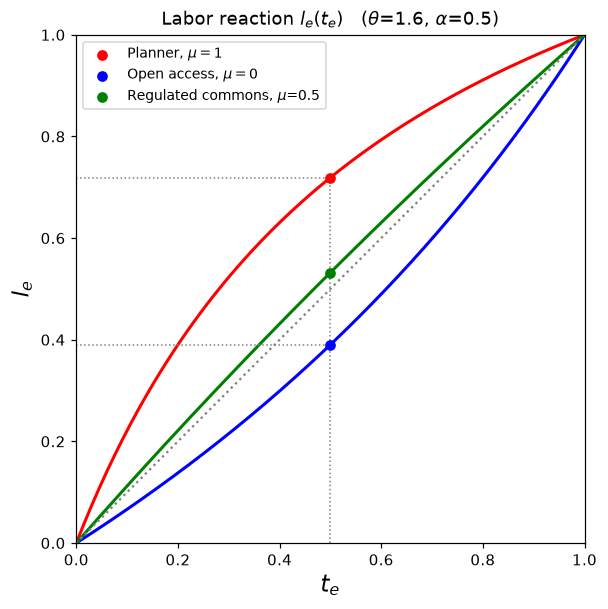
Figure 1:The labor reaction function . The dotted 45° line is — labor and land enclosed in equal proportion. The planner’s curve () bows above it: enclosed land is worked more intensively. Under open access () the curve bows below. The vertical gap between them at any is the labor misallocation that §4.2 is about.
Substituting (4) back into the objective gives output per unit land, equation (5):
This is the step that does the work. What looked like a two-variable optimisation is now a one-dimensional function of , and a concave one.
When should land be enclosed?¶
Because is concave, the planner’s problem is solved by comparing its slope to the enclosure cost . Differentiating and evaluating at the two endpoints gives the parameter thresholds directly.
At , setting and solving for density gives equation (6):
and at , equation (7) — which turns out to be the same locus scaled by :
Below no enclosure is optimal; above full enclosure is; between them, partial. Note the shape of these expressions: every locus is , so a change in costs or productivity shifts all loci vertically by the same amount. That is why the diagrams can be drawn once at without loss.
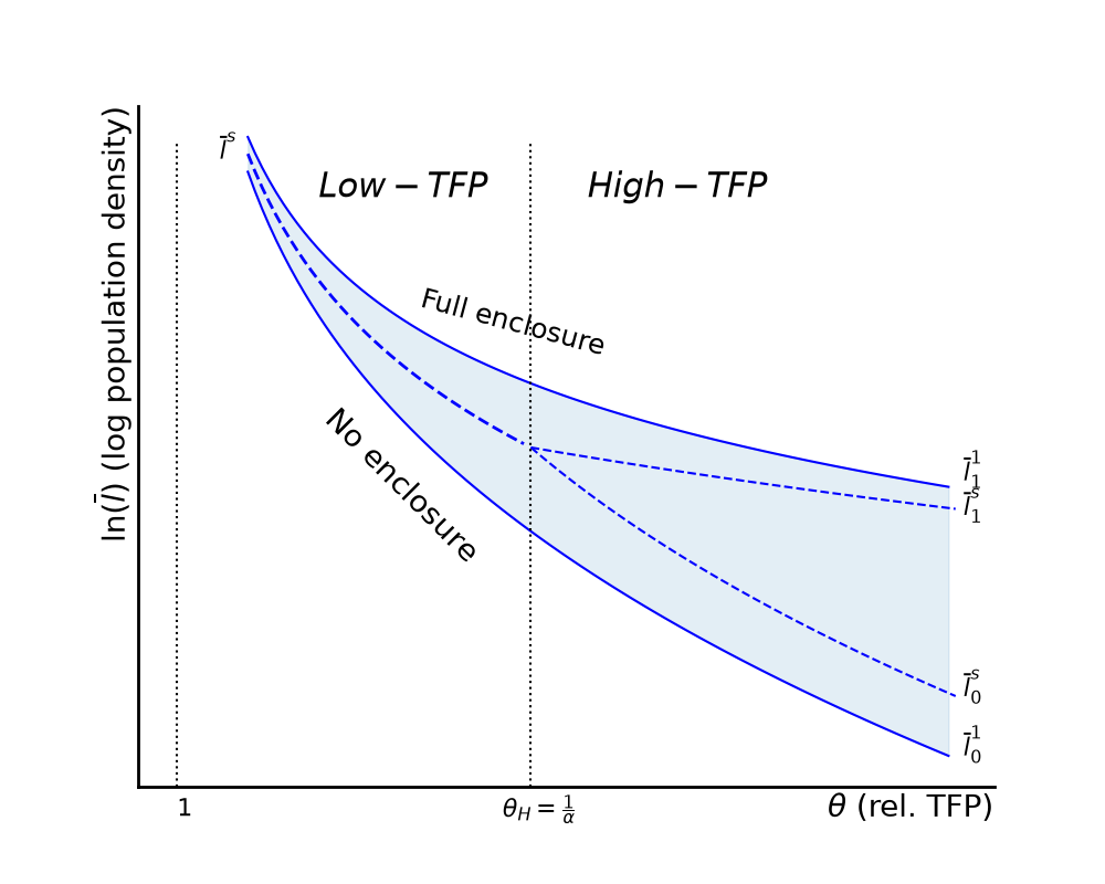
Figure 2:Socially efficient enclosure, in space. The shaded band between and is where partial enclosure is optimal.
The economics is Boserupian: at low density, enclosure costs exceed the gains and the commons persists. Population growth pushes the economy up through , and enclosure begins.
3.3 Decentralized enclosure processes¶
Now replace the planner with private enclosers. The key change is on the commons: labor enters until the average product equals the wage, not the marginal product — the classic open-access distortion, equations (8)–(9).
That single substitution changes and nothing else. The reaction function keeps its form, equation (10), but with
in place of . The inside is the whole distortion.
This immediately explains the threshold that organises the rest of the paper. when , i.e. at
Below , and private enclosure is labor-extensive — enclosing land pushes labor onto the commons. Above it, enclosure is labor-intensive, as the planner’s would be. Almost every qualitative claim in the paper turns on which side of the economy sits.
The private return to enclosing a marginal parcel, equation (12), is
Setting and gives the decentralized thresholds, equations (13)–(14), exactly as before.
3.4 Multiple equilibria and global games¶
Notice the exponent on the bracket. When the bracket decreases in , so increases — enclosure by others raises my return to enclosing. Decisions are strategic complements, and both “nobody encloses” and “everybody encloses” are equilibria. The model has nothing to say about which occurs.
The global-games refinement resolves this. Under Laplacian beliefs an encloser evaluates the expected payoff over uniform on , so the selection condition integrates the return rather than evaluating it at a point:
Carrying out the integral and solving for density gives the risk-dominance locus, equation (15) — the dashed red line in the figures below. Above it, the enclosure cascade tips.
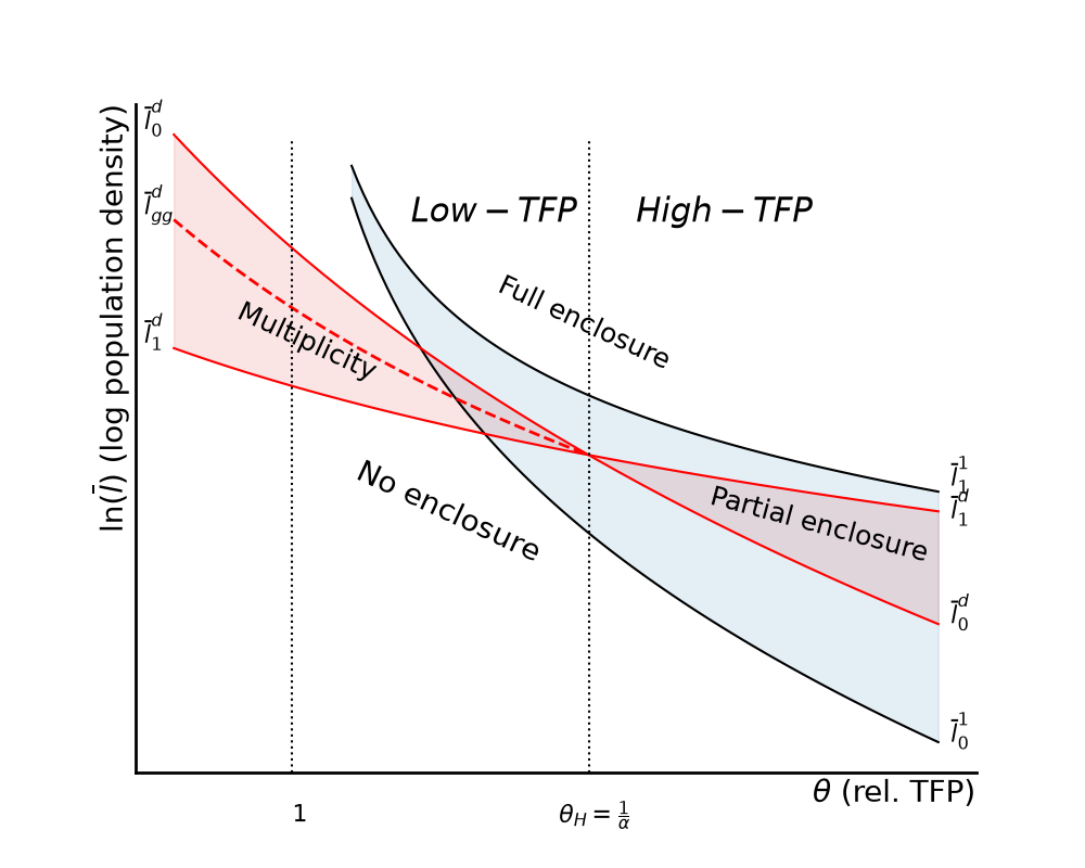
Figure 3:Decentralized enclosure regions (red) against the first-best band (black). The “multiplicity” region left of is where enclosure decisions are strategic complements; selects between the corner equilibria there.
3.5 Comparative statics¶
The loci have a shape worth exploiting. Each one is
so and enter only through the intercept. Halving enclosure costs slides every threshold down by the same — which is geometrically identical to leaving the loci alone and moving the economy’s own point up. Density does exactly that.
So shocks to , and are all the same movement on one fixed canvas, and only and genuinely reshape it. That is what makes a single diagram carry the whole comparative-static story: population growth, cheaper fencing and better baseline technology are one arrow, not three. It is also why no separate figure is needed here — Figures 1 and 2 already show everything, read as a fixed backdrop the economy moves across.
is a third kind, and unlike the others it rescales the axes: , so a more labor-intensive technology shrinks the region below where enclosure decisions are strategic complements. That one you can drag, on the explore page, where the axes visibly move with it while and leave them alone.
4. The social efficiency of private enclosure decisions¶
4.1 Are decentralized enclosures second-best?¶
The comparison that matters is not planner vs. private — the planner also reallocates labor efficiently, which no decentralized process does. The right benchmark is a constrained planner who chooses but must live with the decentralized labor allocation. That gives , equation (17).
behaves differently from in one important way: below it is convex in . So the optimum is at a corner, and finding it means comparing endpoint values rather than solving a first-order condition:
Solving that for density gives , equation (18) — a locus obtained by a genuinely different route from all the others. Above , where is concave again, the usual first-order conditions give equations (19)–(20).
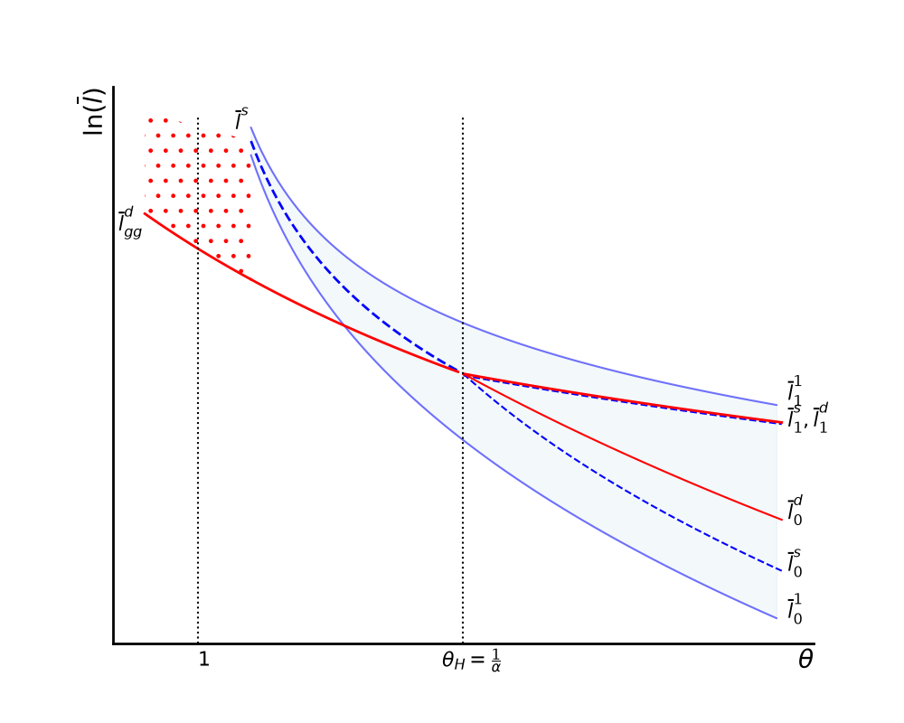
Figure 4:Decentralized outcomes against the second-best. Red hatching (left of ): full enclosure occurs though no enclosure would yield higher net output. Blue hatching (right): too little enclosure, the finer band being a coordination failure.
Two distinct inefficiencies appear, and they point in opposite directions — which is why the paper resists a simple “enclosure is excessive” reading.
4.2 Sources of inefficiency¶
Decomposing the constrained planner’s marginal benefit, equation (21), isolates two things private enclosers ignore.
Displaced rents. The commons is not idle; it yields rents captured by existing users through possession. Enclosers appropriate these without paying for them, so they enclose whenever , even when the net social gain falls short. This drives excessive enclosure.
The labor reallocation gain. On the commons, labor enters until average product equals the wage, pushing below . Enclosure releases workers from that congestion — but enclosers pay the full market wage regardless, so they capture none of the efficiency dividend. This drives insufficient enclosure.
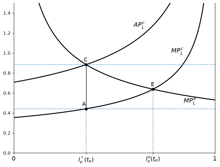
Figure 5:The labor wedge. Commons labor enters until — not — equals the wage, so sits below . The hatched area between and is the efficiency loss enclosure could recover but enclosers are not paid for.
5. The extended model¶
The benchmark assumes an unregulated commons and uncompensated enclosure. Both are extreme. Sections 5.1–5.3 relax them with two parameters, each targeting one of the wedges of §4.2.
5.1 The regulated commons — ¶
Let measure how well the community restrains entry onto the commons. Redoing the labor-allocation condition with that restraint gives equation (23) — and, satisfyingly, it changes nothing except once more:
At this is the open-access ; at it is the planner’s . The single parameter interpolates between the two regimes, which is why the same closed forms carry through the whole extended model.
Since pins the complements/substitutes threshold, governance moves it — equation (24):
falling from at to 1 at . Better governance shrinks the region of multiplicity and dissipative races.
5.2 Power and compensation — ¶
Let be the share of displaced rents an encloser must pay. The enclosure condition becomes , and along the reaction function this is
Compare this with equation (12): the only change is becoming . Every threshold that followed from (12) therefore survives with that one substitution — equations (26)–(27). Integrating this expression over rather than evaluating it at an endpoint gives the -extended global-games locus in the same way as before.
At the locus diverges at : with full compensation, no population density makes enclosure profitable below that productivity gain. This is a statement about profitability, not about expropriation — at nothing is expropriated at all. The paper’s “raid,” the wholly uncompensated taking, is the corner; the divergence here is the opposite corner, where the encloser pays in full and the land is simply not worth the price.
5.3 The extended wedge¶
The two parameters close the two wedges of §4.2, and they close them jointly. Setting makes ; then the identity collapses the decentralized denominator into the planner’s, and the decentralized loci become identical to the first-best ones — not merely close. Neither parameter alone suffices.
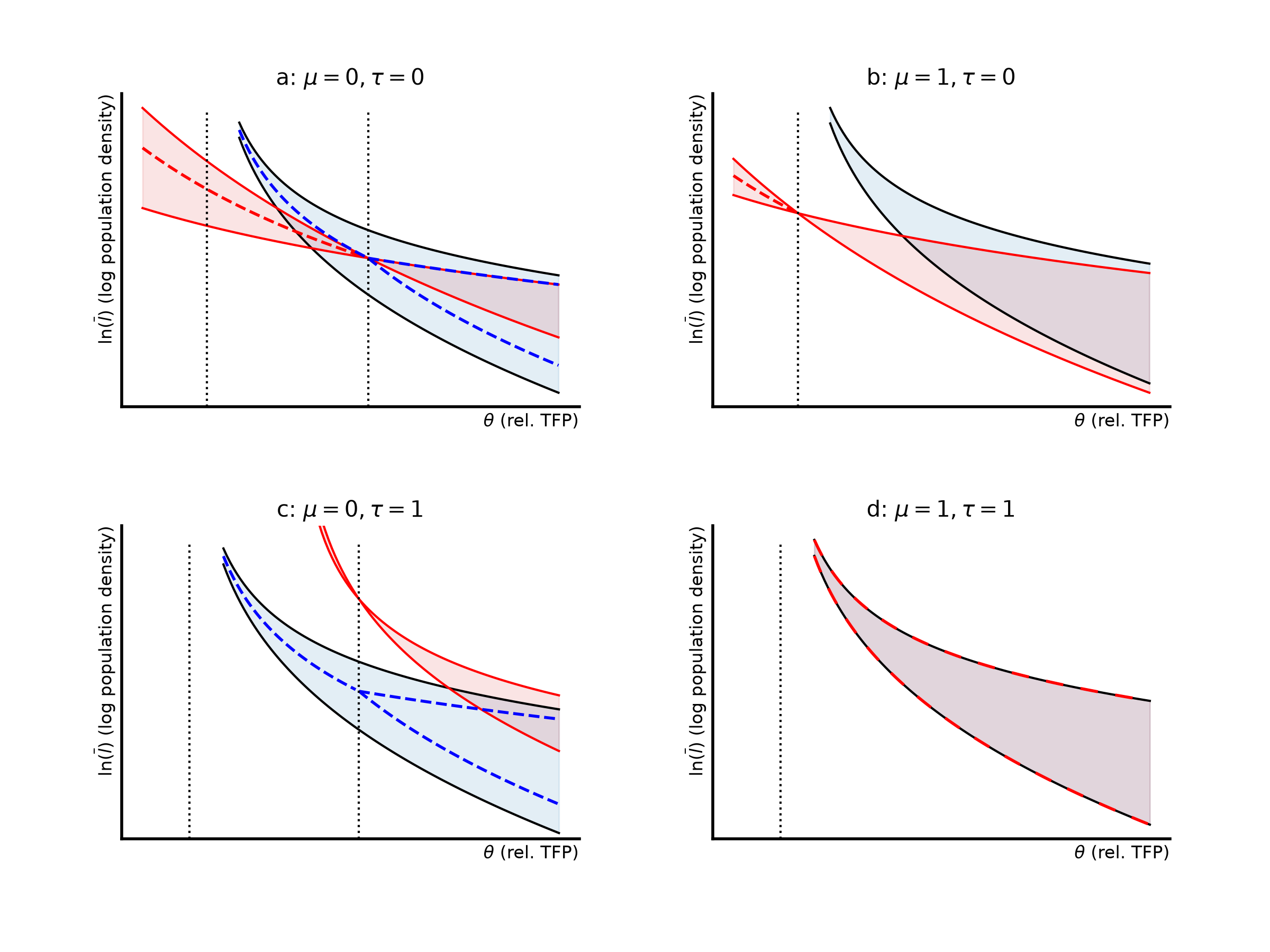
Figure 6:Governance and compensation. (a) the benchmark; (b) alone; (c) alone; (d) both — where the decentralized loci (dashed red) lie exactly on the planner’s (black). They are drawn dashed precisely so the coincidence is visible.
5.4 Power, policy, and the second-best¶
That the wedges close only jointly has a sharp policy reading, and it is the reason the paper resists a simple “strengthen institution X” prescription. Each parameter addresses a different failure:
acts on the labor margin — how well commons land is worked.
acts on the enclosure margin — which land is worth taking.
Fixing one while the other stays broken is a classic second-best problem, and it can leave the economy worse off than fixing neither. Raising alone makes the commons more valuable without making enclosers pay for that value, widening the gap at the full-enclosure margin. Raising alone converts over-enclosure into under-enclosure: transitions that should happen are deterred.
The explore page makes this quantitative — the loss surface has a minimum on the diagonal and rises along both axes.
6. Applications and extensions¶
6.3 Encompassing interests: monopoly enclosure¶
The paper’s §6.3 replaces atomistic enclosers with a single monopolist who internalises the effect of enclosure on the wage. The profit function is formed and differentiated the same way, and the endpoint conditions give the monopoly thresholds, equations (30)–(34).
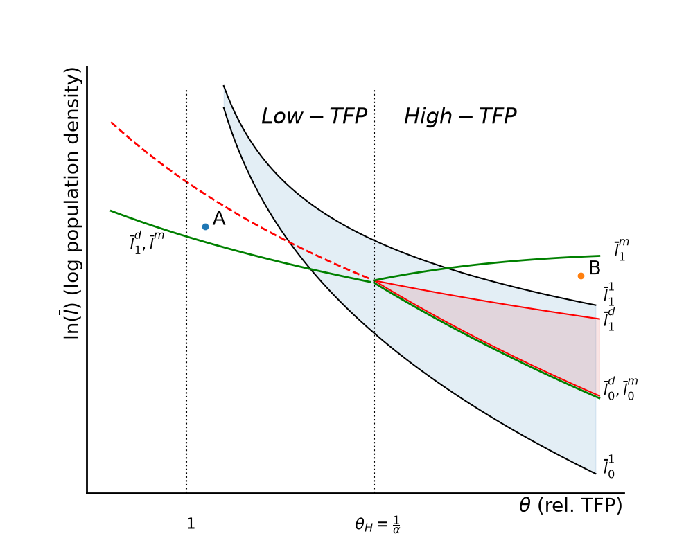
Figure 7:Monopoly enclosure (green) against decentralized (red) and first-best (black).
Where to go next¶
Reproducing the paper’s figures — every figure above, in a few lines of code.
Manufacturing and structural transformation — the three-sector extension, including material developed beyond the published paper.
Mathematical Appendix — the complete derivations, equation by equation.